Applying Neural Architecture Search (NAS) to a real use case

At Preligens, a lot of time and resources are dedicated to R&D. We are part of a team of researchers that strive to apply novel ideas from the literature to real world applications. Neural Architecture Search (NAS) is one of the key subjects we explored in the last few months. We provide in this article a summary of the challenges we encountered, and give some advice to anyone interested in NAS and the use of HPCs for Deep Learning.

NOTE: We also published this paper ! We encourage anyone who is interested in going deeper into the subject to read it.

A little bit of context

Neural Architecture Search

Handcrafting neural networks to find the best performing structure has always been a tedious and time consuming task. Besides, as humans, we naturally tend towards structures that make sense in our point of view, although the most intuitive structures are not always the most performant ones.

NAS is a subfield of Auto-ML that aims at replacing such manual designs with something more automatic. Having a way to make neural networks design themselves would provide a significant time gain, and would let us discover novel, good performing architectures that would be more adapted to their use-case than the ones we design as humans.

The main drawback of this area of research is that it requires a huge amount of computing resources. Proposed approaches in the literature either :

• Generate several architectures based on a blueprint, then train them independently and try to generate an optimal architecture using Reinforcement Learning (RL) or Evolutionary Algorithms (EA) — we call such techniques discrete approaches.
• Generate a densely connected hyper-network with a gigantic amount of parameters, train it, and then decode an optimal sub-network out of it — we call them continuous approaches.

In both cases, it is nearly impossible to get any results in a tractable amount of time without relying on distributed computing. This is also the main reason why this field is not widely studied, as one needs to have access to a lot of computing resources to work on it. Of course, one could also work around the problem by using very small datasets, but that is not possible in a real-world context.

HPC usage

Our project was part of the Grand Challenge Jean-Zay program, initiated by the GENCI, a French civil society dedicated to the provision of supercomputers for open research. For the duration of the project, we were allocated computing hours on a HPC infrastructure called Jean-Zay. The partition of the cluster opened to us owned 351 nodes each equipped with 4 GPUs NVIDIA V100, 2 Intel cascade processors and 192 Gb of RAM.

It was possible for us to simultaneously use up to 512 GPUs for a single training. Exactly the kind of computing power we need for an industrial application of NAS !

Our use-case

We applied NAS on an instance segmentation task, which means we want to distinguish the background of an image from some objects of interest.

In our case, we would like to locate and segment helicopters on satellite images. Our dataset contains publicly available images from the Maxar satellites WorldView 1, 2, and 3, and GeoEye 1, which are tiled into around 18 000 patches of size 512×512.

Some examples from our dataset. Source : Segmentation by Preligens, Satellite images by Maxar

Methods

Before diving into the different approaches proposed in the NAS bibliography, we first need to define some concepts common to all works.

The first element to consider is the operation search space, which is an ensemble of candidate layers (convolutions, poolings…) for our optimal architecture. It must be defined manually and highly depends on the use-case. For example, here is one of the commonly used search spaces from a method named DARTS :

• 3×3, 5×5 Dilated Convolutions
• 3×3, 5×5 Depthwise Separable Convolutions
• 3×3 Average Pooling
• 3×3 Max Pooling
• Skip Connection
• Zero (no connection)

Once our operation search space is defined, we need to consider the structure of our candidate architectures. Usually, in NAS approaches, we define a neural network as a two-staged structure composed of :

• A search network — a directed acyclic graph (DAG) where nodes are search cells
• Many search cells — where edges are associated with an operation from our previously mentioned operation search space

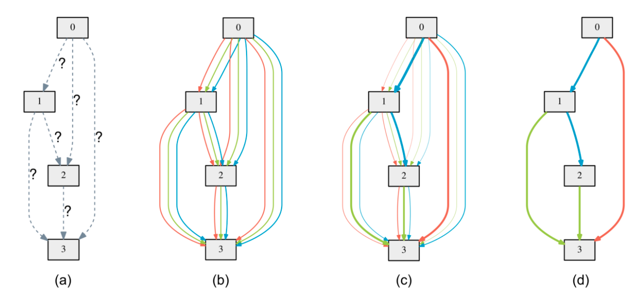
An example of a search network, where each node contains a search cell. Source : Preligens

Initially, we don’t know which operation to associate with each edge. In fact, that is precisely what we are neurally searching for !

Thus, training the search network means finding an optimal operation for all edges of all search cells. In practice, all of our search cells are identical : we only look for a single optimal search cell that we replicate N times.

Once again, network and cell structures must be designed manually and are case-dependent as well. That’s already a lot of decisions to make!

Now that we’ve defined the essential concepts of NAS, let’s jump into the different methods we investigated. The majority of the bibliography we considered can be split into two main families.

Discrete Approaches

Approaches based on the idea of generating an ensemble of candidate architectures from the search space and selecting the optimal one are among the NAS early works.

In this setting, we build several architectures by picking operations to be assigned to edges. Then, we train all generated architectures, and compute a global loss that is used to train a controller, often based on Reinforcement Learning or Evolutionary Algorithms.

While being the most straightforward way of performing NAS, it is also the most expensive in terms of time and computing resources. In fact, first proposed approaches took multiple weeks to train, as just a single pass of RL or EA requires training a handful of neural networks ! We decided to give discrete approaches a try nonetheless.

Continuous Approaches

Taking into account the significant amount of computing resources required for discrete approaches, some works reformulated the problem so that only a single network training is required.

DARTS is the first approach to suggest using continuous relaxation to train a search network. Here, the idea is to build a super-network that encapsulates the whole search space, by assigning a mixed operation to each edge. A mixed operation is simply a weighted sum of all operations contained in the predefined search space. The weights are called α, and are optimized during training (using gradient descent). More precisely, α is a vector which has the same size as the search space, so that each operation is associated with one alpha value.

The DARTS search cell — a mixed operation is symbolized with an ensemble of edges. Source : DARTS Paper

Once the search network is trained, we can decode an optimal structure out of it by selecting the operation tied to the biggest α value. Thus, we achieve the same goal as discrete approaches, but with a single network training. Naturally, this group of approaches is far more performant in terms of training time, the main challenge being the super-network’s size in memory, since the whole search network must fit inside a GPU’s VRAM.

Some other methods, namely PC-DARTS or GAEA came afterwards to solve common problems such as the lack of sparsity among alpha values or a preference towards weight-free operations like pooling that could lead to suboptimal decoded structures. We used them both in our experiments.

Implementation challenges

Building a working NAS framework is really not a piece of cake ! In a nutshell, this is mainly linked to two major factors :

• We want to define complex super-networks and use extremely unorthodox minimization routines
• We need to parallelize computation to perform this search in an acceptable time

As a direct implementation consequence : we end up using mostly experimental sections of the dedicated deep learning backend / library, probably will need to use distributed computing dedicated packages and have to come up with a proper data structuration to encode all theoretical NAS concepts.

Let’s dive into that !

Data structuration : how to put NAS concepts in a codebase ?

The core concept in NAS that needs to be translated into actionable code is the search space. As already mentioned, this can be split into two distinct elements : the DAG that represents all available topologies that can be spawned as classical Neural Networks and the set of operations that can be used in said network.

A natural Python package came to mind to store the DAG encoding : Networkx. It is dedicated to the creation and manipulation of complex networks, and as such provides relevant classes and functions for our needs. In our convention, we chose that each DAG edge will store a tensor, while each node will represent an operation — or cell.

To store the set of operations, we used two simple dictionaries : one mapping each layer name to its library implementation, and a second one storing default parameterization for each of these layers. Of course, the second one is used as generic and all parameters for our experiments are specified using a dedicated yaml file provided to our script.

Upon using these two ideas, you can very simply instantiate any network part of your search space by :

• Looping through your nodes in topological order
• Look up for your relevant node operands in the list
• Instantiate the layer using your mapping dictionary
• And apply it to your input tensors !

Tasks parallelism for discrete distribution

As previously explained, discrete methods proceed by generating / testing batches of architectures following a specific exploration strategy. Keeping that in mind, we can therefore speed this process up by exploiting task parallelism : for each batch, a process will act as an orchestrator, dispatching computations to every available GPUs.

MPI (Message Passing Interface) is a library massively used on HPC worldwide, and is a very good tool for this purpose. Our framework being coded in Python, we relied on a dedicated package : MPI4Py.

Of course, all trainings will be handled asynchronously : each training step time varies heavily following the architecture complexity. To take this into account, the orchestrator will handle workload synchronization though peer to peer communication. Upon creating the MPI communicator mpi_com — MPI.COMM_WORLD — this communication is handled through the functions mpi_com.send() and mpi_com.recv(). Thanks to the orchestrator, we do not need to use any barrier.

More details can be found in the paper, but the general parallelism through orchestrator dispatching follows the logic presented in the following figure.

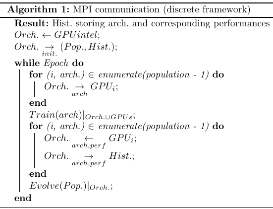
Computations orchestration principal of our discrete framework. Source : Preligens

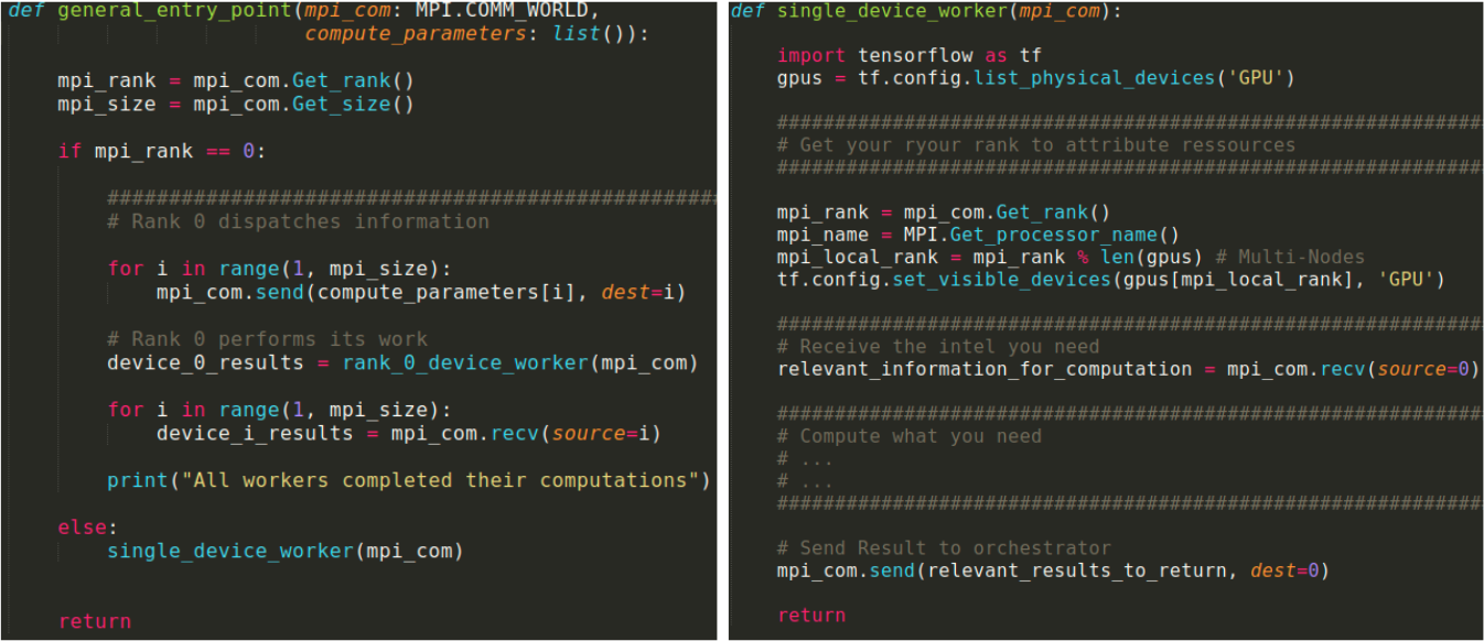
Pseudo-code of computation dispatching using MPI4py. Source : Preligens

A very important point to take into consideration : do be careful with your import tensorflow ! In many deep learning codebases using Tensorflow framework, this import can be found in multiple files. This instruction however triggers library opening / loading — such as CUDNN — and can cause conflicts and terminate code execution when used in multi-GPUs context.

Following the dispatch presented here, this is easily handled by strictly containing these imports at child process level ! It’s always good to know, as one may have to restructure an entire codebase if not aware of this detail !

Data parallelism for continuous distribution

Training continuous approaches using distributed computing is far more straightforward than the discrete ones, as we rely on data parallelism.

Here, as we simply need to train a single search network, we can apply this classical distribution paradigm that is supported by most deep learning frameworks (namely Tensorflow and PyTorch). The idea is to replicate the whole neural network and distribute a shard of data on each GPU available. For example, with a batch size of 64 and 8 GPUs, each GPU will handle a mini-batch of 8. Once the forward pass is done, a synchronization is necessary on the backward pass to compute a global loss and apply a global gradient on all instances of the network : we need to make sure each copy of the network is identical.

An illustration of data parallelism. Each model replica handles a data shard and global updates are performed. Source : Quora

When using an HPC, it is important to distinguish between two cases :

• The usage of multiple GPUs on a single node, that we call mono-node/multi-gpu
• The usage of multiple GPUs on multiple nodes, that we call multi-node/multi-gpu

The latter is obviously more challenging since a communication between different nodes (i.e machines) needs to be established. Usually, this communication is performed using MPI.

As we relied on Tensorflow for this project, we first explored the dedicated libraries : tf.distribute.MirroredStrategy (mono-node/multi-gpu) and tf.distribute.experimental.MultiWorkerMirroredStrategy (multi-node/multi-gpu). We needed to handle both cases, so we worked with the most generic one and implemented our framework using MultiWorkerMirroredStrategy. Did you notice the “experimental” in the package name ? This is where the fun begins.

In our multi-node/multi-gpu setting, we encountered synchronization problems (i.e stuck training), and the code setup was no easy task, even following the official documentation. Furthermore, it was hard to find any clue on how to solve the problem, since few resources were available online, and no error log was displayed. Finally, a lot of things are done “under the hood”, especially MPI communication, which makes it even harder to understand what is going on.

After a long discussion with Jean-Zay’s support team (many thanks to them !), we decided to switch to Horovod. It is a framework dedicated to distributed computing, which supports both Tensorflow and PyTorch. Like Tensorflow’s MultiWorkerMirroredStrategy, it is based on MPI to establish communication between nodes. Unlike the former, one needs to handle some subtleties tied to MPI such as worker ranking. Thus, to use Horovod, it is necessary to understand some basic MPI concepts, but integrating the framework in an existing codebase remains easy and can be done in a short amount of time (in fact, it only took us a single day !).

We managed to solve all our problems by replacing MultiWorkerMirroredStrategy with Horovod, besides some isolated failures that only happened once.

What can we learn from this experience ? In a mono-node/multi-gpu context, using Tensorflow’s MirroredStrategy is fine. In a multi-node/multi-gpu context, we strongly advise using Horovod instead of TensorFlow’s MultiWorkerMirroredStrategy.

Horovod is a backend-agnostic framework for distributed computing in deep learning.

In short : don’t trust experimental packages !

Experiments & Results

Most of our experiments consisted in building a U-Net network topology based on DARTS cells, eventually we also compared different ways to build the cell topology (how the nodes within the cells are connected). In this post, we only comment on the most important observations that we had.

Mitigated Results

Throughout our experiments, we never managed to reach performance levels really close to what we could obtain with a production proofed architecture. It can be a bit rewarding to see that human efforts invested in optimizing the model’s structure really paid off, though we were optimistic to reach high levels of performance with NAS. In the following figure, one can observe the precision-recall curve for several IoU thresholds for two models. The baseline model corresponds to the production grade architecture, while the ResNeXt-UNet is a U-Net-like structure composed of ResNeXt type cells.

It is quite clear that a gap is maintained between the two models as we were not able to reach better performance with the DARTS approach. This led us to question whether the method is really effective.

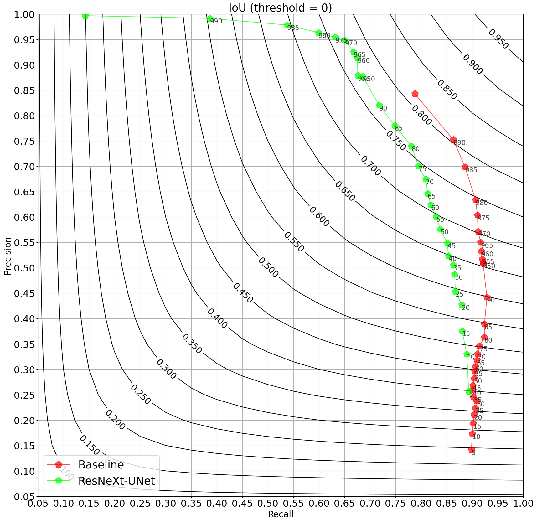
Precision-recall curves for our NAS-found architecture and a production-type baseline. Source : Preligens

You always need a baseline

Because the DARTS approach did not perform as expected, we decided to benchmark this NAS method against a simpler version : a basic random search. It only consists in randomly selecting operations with a cell and connecting them to have a functional block that fits as a replacement to the DARTS cell. Simply put, the job normally done by DARTS is replaced by randomly selecting the operations and connections.

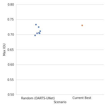
Comparison between NAS-found structure and randomly sampled ones. Source : Preligens

After running this random search step several times, we obtained candidate architectures that we finally trained in the same way as DARTS. The previous figure details the maximum IoU that we obtained after this last training step. It shows that the best candidate found with DARTS basically exhibits a similar IoU performance to what we can find with a few random tries. These final experiments helped us to realize that this technology is probably not mature enough to provide the performance jump that we expected.

Conclusion

This first batch of experiments enabled us to gain an in-depth understanding of core NAS technologies and dedicated implementation tricks, and we once again thank GENCI for their Grand Challenge project that provided us with the required hardware to do so.

In these experiments, we haven’t yet managed to outperform our handcrafted and tailored architectures. This objective was however really ambitious using our current framework as we couldn’t achieve such a level of architecture tuning — e.g. multiple cells adaptation. On the good side, the tool managed to obtain not so bad structures in matters of hours : this in itself is satisfactory when one compares the time involved to handcraft a well behaving network structure.

In terms of transferability to real complex use-cases, it is our current opinion that NAS is not yet mature enough. Indeed, proposed methods require the use of more hyper parameters than classical deep learning and the optimization schemes are much more challenging in terms of proper convergence.

Moreover, one cannot rely on pre-trained structures — e.g. ImageNet weights — and therefore random initialization of all weights in the super-network have a large impact on ultimate mean IOU achieved. Another point of concern regarding this technology : it is still not clear that NAS manages to outperform random search by a significant margin. This point is often mentioned in the literature and questions the relevance of NAS approaches.

For further studies related to this topic, we therefore think about two axes that could address part of these concerns. The first one would be to devise a metric to assess network structural soundness before any search / training phase : using it, one could remove the evaluation bias linked to the network weight and really focus attention on the probed topology. The second one would be to reduce the problem complexity in order to better condition the search phase : for example one could think about only searching / improving a subpart of an already well designed architecture. Some preliminary results also made us think about a tool that could be used to locate which parts of the considered network should be improved first.